Alternating Sign Matrices

The Remarkable Sequence 1, 2, 7, 42, 429, ...: The story of Alternating Sign Matrices

Manjil Saikia

Jun 7, 2018 • 11 min read

The sequence in the title is given by the following ‘nice’ formula ${\frac{1!4!7!\cdots (3n-2)!}{n!(n+1)!\cdots (2n-1)!}}$ or, in product notation ${\prod_{j=0}^{n-1}\frac{(3j+1)!}{(n+j)!}.}$ Here ${k!}$ denotes the product ${1\cdot 2 \cdot 3\cdots k}$ . This formula was conjectured by Mills, Robbins and Rumsey to count what are called alternating sign matrices (ASMs), which is the subject of this post.

An alternating sign matrix (ASM) of size n is an ${n \times n}$ matrix with entries in the set ${ \{0, 1, -1\}}$ such that

(i) all row and column sums are equal to 1,

(ii) and the non-zero entries alternate in each row and column.

For instance, there are 7 ASMs of order 3, these are the six permutation matrices (which are matrices with entries either ${1}$ or ${0}$ such that only one ${1}$ appears in each row and each column) and the matrix

$\displaystyle \begin{pmatrix}0&1&0\\1&-1&1\\0&1&0\end{pmatrix}.$

By the definition of an ASM it is clear that all permutation matrices are ASMs (why?).

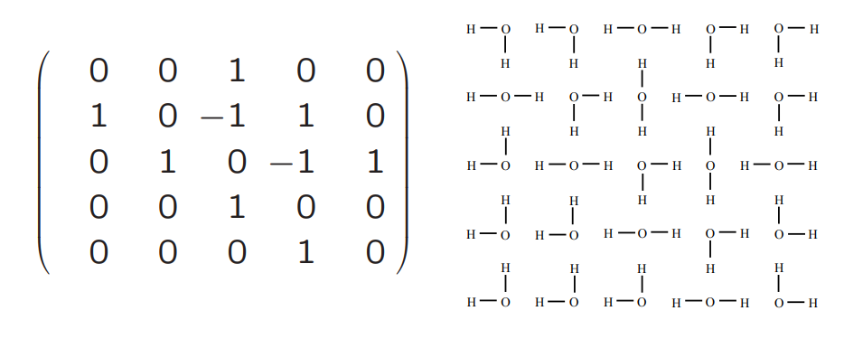
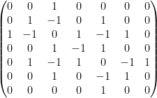
An example of a bigger ASM is given below.

$\displaystyle \begin{pmatrix}~~0&~~0&~~0&~~1&~~0&~~0&~~0\\~~0&~~1&~~0&-1&~~0&~~1&~~0\\~~1&-1&~~0&~~1&~~0&-1&~~1\\~~0&~~0&~~1&-1&~~1&~~0&~~0\\~~0&~~1&-1&~~1&-1&~~1&~~0\\~~0&~~0&~~1&-1&~~1&~~0&~~0\\~~0&~~0&~~0&~~1&~~0&~~0&~~0\end{pmatrix}$

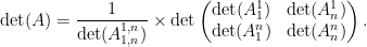
But, how were these matrices first defined? Let zs start with the determinants, that we all know. For example, for the matrix

$\displaystyle \begin{pmatrix}a&b\\c&d\end{pmatrix}$

the determinant is ${ad-bc.}$ And similarly, for the matrix

$\displaystyle \begin{pmatrix}a&b&c\\d&e&f\\g&h&i\end{pmatrix}$

the determinant is ${aei+bfg+cdh-ceg-bdi-afh.}$

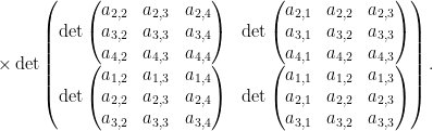
We can keep on doing this and more generally, for an ${n\times n}$ matrix, ${A}$ with entries ${a_{i,j}}$ ${(1\leq i,j\leq n)}$ , the determinant of ${A}$ is defined as

$\displaystyle \textup{det}(A)=\sum_{\sigma \in S_n}\textup{sgn} (\sigma)\prod_{i=1}^{n}a_{i,\sigma(i)}.$

Given a matrix ${A}$ , we let ${A^i_j}$ denote the matrix that remains when the ${i}$ th row and ${j}$ th column of ${A}$ are deleted. If we remove more than one row or column, then the indices corresponding to those are added to the super- and sub- scripts.

Theorem 1 (Desnanot-Jacobi adjoint matrix theorem) If ${A}$ is an ${n\times n}$ matrix, then

$\displaystyle \det(A)\det(A^{1,n}_{1,n})=\det(A^1_1)\det(A^n_n)-\det(A^1_n)\det(A^n_1)$

or

$\displaystyle \det(A)=\frac{1}{\det(A^{1,n}_{1,n})} \times \det \begin{pmatrix} \det (A^1_1)& \det (A^1_n)\\ \det (A^n_1)& \det(A^n_n)\end{pmatrix}.$

This gives us a way of evaluating determinants, in terms of smaller determinants. Reverend Charles L. Dodgson, better known by his pen name of Lewis Carroll used the Desnanot-Jacobi theorem to give an algorithm for evaluating determinants in terms of ${2\times 2}$ determinants.

For instance, we get

${\det\begin{pmatrix}a_{1,1}&a_{1,2}&a_{1,3}&a_{1,4}\\a_{2,1}&a_{2,2}&a_{2,3}&a_{2,4}\\a_{3,1}&a_{3,2}& a_{3,3}&a_{3,4}\\a_{4,1}&a_{4,2}&a_{4,3}&a_{4,4}\end{pmatrix}=\frac{1}{\det \begin{pmatrix} a_{2,2}&a_{2,3}\\a_{3,2}&a_{3,3} \end{pmatrix}}}$

$\displaystyle \times \det \begin{pmatrix} \det \begin{pmatrix} a_{2,2}&a_{2,3}&a_{2,4}\\a_{3,2}&a_{3,3}&a_{3,4}\\a_{4,2}&a_{4,3}&a_{4,4} \end{pmatrix} & \det \begin{pmatrix} a_{2,1}&a_{2,2}&a_{2,3}\\a_{3,1}&a_{3,2}&a_{3,3}\\a_{4,1}&a_{4,2}&a_{4,3}\end{pmatrix}\\ \det \begin{pmatrix} a_{1,2}&a_{1,3}&a_{1,4}\\a_{2,2}&a_{2,3}&a_{2,4}\\a_{3,2}&a_{3,3}&a_{3,4} \end{pmatrix}& \det \begin{pmatrix} a_{1,1}&a_{1,2}&a_{1,3}\\a_{2,1}&a_{2,2}&a_{2,3}\\a_{3,1}&a_{3,2}&a_{3,3} \end{pmatrix}\end{pmatrix}.$

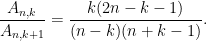
In the 1980s, Robbins and Rumsey looked at a generalization of the ${2\times 2}$ determinant, which they called the ${\lambda}$ -determinant. They defined

$\displaystyle \textup{det}_\lambda \begin{pmatrix}a_{1,1}&a_{1,2}\\a_{2,1}&a_{2,2}\end{pmatrix}=a_{1,1}a_{2,2}+\lambda a_{2,1}a_{1,2}.$

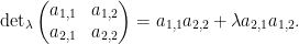
Using the previous observations, they generalized it to an ${n\times n}$ determinant. Their main result in this direction was

Theorem 2 (Robbins-Rumsey) Let ${A}$ be an ${n\times n}$ matrix with entries ${a_{i,j}}$ , ${\mathcal{A}_n}$ be the set of all ASMs, ${\mathcal{I}(B)}$ be the inversion number of ${B}$ and ${\mathcal{N}(B)}$ be the number of ${-1}$ ‘s in ${B}$ . Then

$\displaystyle \textup{det}_\lambda(A)=\sum_{B\in \mathcal{A}_n}\lambda^{\mathcal{I}(B)}(1+\lambda^{-1})^{\mathcal{N}(B)}\prod_{i,j=1}^na_{i,j}^{B_{i,j}}.$

This was the first appearance of an ASM in the literature.

What is the inversion number of an ASM? An easy way to calculate the inversion number is to take products of all pairs of entries for which one of them lies to the right and above the other, and then adding them all up.

$\displaystyle \begin{pmatrix}0&1&0&0&0\\0&0&1&0&0\\1&-1&0&0&1\\0&1&-1&1&0\\0&0&1&0&0\end{pmatrix}$

In the matrix above, there are seven pairs here whose product is ${+1}$ and two pairs whose product is ${-1}$ . So the inversion number is ${5}$ .

Let us now make some observations, we look at an ASM below.

$\displaystyle \begin{pmatrix}0&0&1&0\\0&1&0&0\\1&-1&0&1\\0&1&0&0 \end{pmatrix}$

There can be only one ${1}$ in the top row (or, first column). Let ${A_{n,k}}$ be the number of ${n\times n}$ ASMs with a ${1}$ at the top of top ${k}$ th column. Some thought will give us, ${A_{n,k}=A_{n, n+1-k}}$ (symmetry). Further, if ${A_n}$ is the number of ${n\times n}$ ASMs, then ${A_{n,1}=A_{n,n}=A_{n-1}}$ . This allows one to check small values to get a formula. Mills, Robbins and Rumsey did exactly that. They first conjectured

$\displaystyle \frac{A_{n,k}}{A_{n,k+1}}=\frac{k(2n-k-1)}{(n-k)(n+k-1)}.$

This means that the ${A_{n.k}}$ ‘s are uniquely determined by the ${A_{n,k-1}}$ ‘s when ${k>1}$ and by ${A_{n,1}=\sum_{k=1}^{n-1}A_{n-1,k}}$ . The above conjecture can be reformulated as

$\displaystyle A_{n,k}=\binom{n+k-2}{k-1}\frac{(2n-k-1)!}{(n-k)!}\prod_{j=0}^{n-2}\frac{(3j+1)!}{(n+j)!}.$

From here, knowing that ${A_{n}=A_{n+1,1}}$ allows one to conjecture the formula we had in the beginning.

But, what about a proof? Doron Zeilberger succeeded in proving the formula (called the ASM conjecture) in 1996 using constant term identities. The proof ran for 84 pages and involved a team of referees to check all the details. Shortly after, Greg Kuperberg gave an alternate proof by exploiting a connection between ASMs and statistical physics. It turned out that physicists have been studying ASMs under a different guise.

In the above picture, we see an ASM on the left and a model called the square ice model on the right. To each entry in an ASM we assign one of the six possibilities of arrangement of the water molecules on the right such that the angle between a ${H-O-H}$ bond is either ${90}$ or ${180}$ degrees. We leave it to the reader to see that this is indeed a bijection.

In the late 1980’s Richard Stanley suggested the study of various symmetry classes of ASMs; this let Robbins to conjecture formulas for many of these classes. It turned out to be as difficult as enumrating ASMs, and this study was only recently completed in 2016.

(i) Vertically Symmetric ASMs: ${a_{i,j}=a_{i,n+1-j}}$ , ${n}$ odd (Kuperberg 2002)

(ii) Half-turn Symmetric ASMs: ${a_{i,j}=a_{n+1-i,n+1-j}}$ , ${n}$ odd (Razumov-Stroganov 2005), ${n}$ even (Kuperberg 2002)

(iii) Diagonally Symmetric ASMs: ${a_{i,j}=a_{j,i}}$ , no ‘nice’ formula

(iv) Quarter-turn Symmetric ASMs: ${a_{i,j}=a_{j,n+1-i}}$ , ${n}$ odd (Razumov-Stroganov 2005), ${n}$ even (Kuperberg 2002)

(v) Horizontally and vertically Symmetric ASMs: ${a_{i,j}=a_{i,n+1-j}=a_{n+1-i,j}}$ , ${n}$ odd (Okada 2004)

(vi) Diagonally and Antidiagonally Symmetric ASMs: ${a_{i,j}=a_{j,i}=a_{n+1-j,n+1-i}}$ , ${n}$ odd (Behrend-Fischer-Konvalinka 2017)

(vii) All symmetries: ${a_{i,j}=a_{j,i}=a_{i,n+1-j}}$ , no ‘nice’ formula.

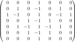
Here is an example of a vertically symmetric ASM.

$\displaystyle\begin{pmatrix}~~0&~~0&~~0&~~1&~~0&~~0&~~0\\~~0&~~1&~~0&-1&~~0&~~1&~~0\\~~1&-1&~~0&~~1&~~0&-1&~~1\\~~0&~~0&~~1&-1&~~1&~~0&~~0\\~~0&~~1&-1&~~1&-1&~~1&~~0\\~~0&~~0&~~1&-1&~~1&~~0&~~0\\~~0&~~0&~~0&~~1&~~0&~~0&~~0\end{pmatrix}$

Are ASMs worth studying only because they are difficult to enumerate? The answer is of course a big NO! They are intimately related to other objects that combinatorialists study. We give a few examples.

A plane partition in an ${a\times b \times c}$ box is a subset ${PP\subset \{1,2,\cdots, a\}\times \{1,2,\cdots, b\}\times \{1,2, \cdots, c\}}$ with ${(i^\prime, j^\prime, k^\prime)\in PP}$ if ${(i,j,k)\in PP}$ and ${(i^\prime, j^\prime, k^\prime)\leq (i,j,k)}$ . We usually denote them by a pictorial description, where each entry of the set corresponds to a box. An example is shown below.

A plane partition in an ${n\times n \times n}$ box is called cyclically symmetric if ${(j,k,i)\in PP}$ when ${(i,j,k)\in PP}$ . George Andrews in 1979 proved that the number of cyclically symmetric plane partitions in an ${n \times n \times n}$ box is ${\prod_{j=0}^{n-1}\frac{(3j+2)(3j)!}{(n+j)!}.}$ An example is given below.

We state only two instances where plane partitions and ASMs appear together.

Theorem 3 (Ayyer-Behrend-FIscher) The number of ${2n+1 \times 2n+1}$ diagonally and antidiagonally symmetric ASMs (DADSASMs) with ${n+1}$ occurences of ${1}$ ‘s in the diagonals and antidiagonals in their fundamental region is equal to the number of cyclically symmetric plane partitions in an ${n \times n \times n}$ box.

An example of a DADSASM is given below.

$\displaystyle \begin{pmatrix}0&0&1&0&0&0&0\\0&1&-1&0&1&0&0\\1&-1&0&1&-1&1&0\\0&0&1&-1&1&0&0\\0&1&-1&1&0&-1&1\\0&0&1&0&-1&1&0\\0&0&0&0&1&0&0\end{pmatrix}$

If a plane partition has all the symmetries and is its own complement, then it is called totally symmetric self-complementary plane partitions. For, instance the following is one.

This class of plane partitions inside a ${2n \times 2n \times 2n}$ box are equinumerous with ${n \times n}$ ASMs!

Another object which is related to ASMs is alternating sign triangles (ASTs), An AST of size ${n}$ is a triangular array such that

(i) the entries are either ${1, -1}$ or ${0}$ ,

(ii) along the columns and rows the non-zero entries alternate,

(iii) the first non-zero entry from the top is a ${1}$ and the rowsums are equal to ${1}$ .

A recent theorem is the following.

Theorem 4 (Ayyer-Behrend-Fischer) The number of ASMs of size ${n}$ is equal to the number of ASTs of order ${n}$ .

There are other combinatorial objects which are equinumerous with ASMs, and one of the major open problems in enumerative combinatorics is to find bijections between such objects. The object of this post was to give a very brief introduction to ASMs, which are beautiful combinatorial objects that are studied by mathematicians in many different ways. A good place to start reading about them is the book Proofs and Confirmations by David Bressoud.

Sign up for more like this.