Basics of Non-Linear Dynamics

Look around and you will observe that all physical systems around us are dynamical in nature. That is, any system whose status changes with time is Dynamical. Whether the system in question keeps repeating itself (like in the case of an un-damped simple pendulum), or settles down to equilibrium (some population models) or does something more complicated (for instance Lorentz system), the dynamics of the system is used to analyze its behavior.

To mathematically define the dynamics of a given system, we specify how the `states’ change with time and that gets expressed in the form of Differential Equations. We then define a space, with `states as the coordinates’ called the State Space or Phase Space. It is thus easy to graphically visualize dynamics as trajectories in the state space.

Simple trajectories are obtained by linear differential equations. But most systems found in nature are inherently non-linear; linearity being a special case. Non-linear systems may exhibit many types of complex dynamical behaviours. A beautiful example given by Prof Steven Strogatz in his book on Non-Linear Dynamics is {to try listening to two of your favorite songs simultaneously and not surprisingly, it does not give you twice the pleasure! The principle of super-position fails spectacularly.

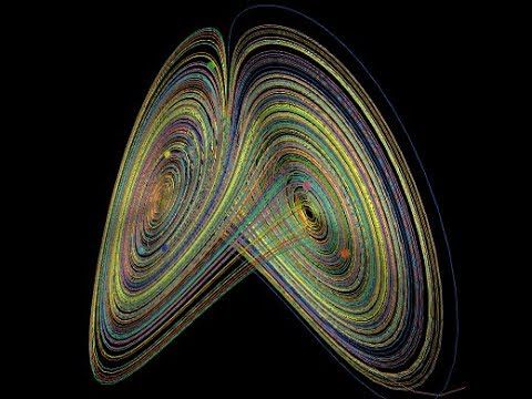
Chaos Image via Shutterstock

Chaos is a very interesting example of a non-linear dynamical system. In both scientific jargon as well as in the layman’s language it denotes random and unpredictable behavior. Technically it is deterministic with long term aperiodic behaviour and exhibits sensitivity dependence on initial conditions. Fancy as it may sound all it means is that, if you start of with two initial conditions no matter how close they are to each other in a chaotic system, the trajectories will diverge from each other at a rate characteristic of the system and bear no resemblance to each other. As in the case of Butterfly Effect, where even small perturbations like the flapping of wings by the butterfly can lead to significantly deviation from the expected outcome. Chaos is deterministic in principle because given the initial conditions are known with infinite accuracy the trajectory of the system can be quantitatively determined. Since the initial conditions can only be known with finite accuracy hence the long term prediction is nearly impossible.

The theory of chaos as summarized by Edward Lorenz is, ‘‘When the present determines the future, but the approximate present does not approximately determine the future.”

The analytical solutions to non-linear differential equations are difficult to be obtained, therefore pictures (phase portraits) come in as creative tools to analyze the dynamic behavior. To find the solution to $$x^{prime}=f(x)$$ starting from an arbitrary initial condition x0, we place an imaginary particle (known as phase point) at x0 and track its pathway along the flow. As time goes on, the phase point moves along the x-axis according to some function x(t). This function is called the Trajectory, based at x0, and it represents the solution of the differential equation starting from that initial condition. A picture which shows all the qualitatively different trajectories of the system is called a Phase Portrait.

The appearance of the phase portrait is controlled by the fixed points x*, defined by f(x*) = 0. In terms of original differential equations, the fixed points represent equilibrium solutions. An equilibrium is said to be stable if all sufficiently small disturbances away from it damp out in time. Thus stable fixed equilibria correspond to stable fixed points. Disturbances grow in time in an unstable equilibrium.

We establish another interesting concept of Linear Stability Analysis for differential equations to get a more quantitative behaviour around the fixed points than the geometrical method. We look at the local neighbourhood around the equilibrium points and in this neighbourhood we can locally linearise it using the Jacobian Matrix. It gives a more mathemathical idea of how the perturbations around a fixed point would grow or decay exponentially or swing in cycles.

The science of Chaos is relatively new and interesting with diverse and extensive application. It was first popularized by James Gleick in 1989, in his book ‘Chaos-Making a New Science’ but it was only in the 1960’s that Lorentz used the theory to accurately model the weather system. The experiment was found to be futile due to the complex nature of chaos and non linear equations. Although difficult to be resolved, nonlinear systems are central to chaos theory and often exhibit fascinatingly complex and chaotic behavior. It is widely applied for studying population growth models, meteorology and circuits like Chua’s circuits etc.